Databricks Auto Scaling</span> Best Practices for Cost Control</a></h1> </div> </div> </div> </div> <div class="elementor-element elementor-element-71e89ea e-flex e-con-boxed e-con e-parent" data-id="71e89ea" data-element_type="container"> <div class="e-con-inner"> <div class="elementor-element elementor-element-ca36d80 e-con-full e-flex e-con e-child" data-id="ca36d80" data-element_type="container"> <div class="elementor-element elementor-element-8129889 e-con-full e-flex e-con e-child" data-id="8129889" data-element_type="container" data-settings="{"background_background":"classic"}"> <div class="elementor-element elementor-element-c5470a3 elementor-widget elementor-widget-text-editor" data-id="c5470a3" data-element_type="widget" data-widget_type="text-editor.default"> <div class="elementor-widget-container"> <p>Author:</p> </div> </div> <div class="elementor-element elementor-element-37a3d4a elementor-position-left elementor-position-left elementor-vertical-align-middle elementor-widget elementor-widget-image-box" data-id="37a3d4a" data-element_type="widget" data-widget_type="image-box.default"> <div class="elementor-widget-container"> <div class="elementor-image-box-wrapper"><figure class="elementor-image-box-img"><a href="https://dateonic.com/author/kamildateonic-com/" tabindex="-1"><img width="512" height="512" src="https://dateonic.com/wp-content/uploads/2025/02/149071.png" class="attachment-full size-full wp-image-1938" alt="" /></a></figure><div class="elementor-image-box-content"><p class="elementor-image-box-title"><a href="https://dateonic.com/author/kamildateonic-com/">Kamil Klepusewicz</a></p><p class="elementor-image-box-description">Software Engineer</p></div></div> </div> </div> <div class="elementor-element elementor-element-f25e5b8 elementor-widget elementor-widget-text-editor" data-id="f25e5b8" data-element_type="widget" data-widget_type="text-editor.default"> <div class="elementor-widget-container"> <p>Date:</p> </div> </div> <div class="elementor-element elementor-element-24b50df elementor-align-left elementor-widget__width-inherit elementor-widget elementor-widget-post-info" data-id="24b50df" data-element_type="widget" data-widget_type="post-info.default"> <div class="elementor-widget-container"> <ul class="elementor-inline-items elementor-icon-list-items elementor-post-info"> <li class="elementor-icon-list-item elementor-repeater-item-4208b33 elementor-inline-item" itemprop="datePublished"> <span class="elementor-icon-list-text elementor-post-infoitem elementor-post-infoitem--type-date"> <time>16 czerwca, 2026</time> </span> </li> </ul> </div> </div> </div> <div class="elementor-element elementor-element-8bef8a6 elementor-toc--minimized-on-tablet elementor-widget elementor-widget-table-of-contents" data-id="8bef8a6" data-element_type="widget" data-settings="{"exclude_headings_by_selector":[],"no_headings_message":"No headings were found on this page.","headings_by_tags":["h2","h3","h4","h5","h6"],"marker_view":"numbers","minimize_box":"yes","minimized_on":"tablet","hierarchical_view":"yes","min_height":{"unit":"px","size":"","sizes":[]},"min_height_tablet":{"unit":"px","size":"","sizes":[]},"min_height_mobile":{"unit":"px","size":"","sizes":[]}}" data-widget_type="table-of-contents.default"> <div class="elementor-widget-container"> <div class="elementor-tocheader"> <h4 class="elementor-tocheader-title"> Table of Contents </h4> <div class="elementor-toctoggle-button elementor-toctoggle-button--expand" role="button" tabindex="0" aria-controls="elementor-toc8bef8a6" aria-expanded="true" aria-label="Open table of contents"><svg aria-hidden="true" class="e-font-icon-svg e-fas-chevron-down" viewBox="0 0 448 512" xmlns="http://www.w3.org/2000/svg"><path d="M207.029 381.476L12.686 187.132c-9.373-9.373-9.373-24.569 0-33.941l22.667-22.667c9.357-9.357 24.522-9.375 33.901-.04L224 284.505l154.745-154.021c9.379-9.335 24.544-9.317 33.901.04l22.667 22.667c9.373 9.373 9.373 24.569 0 33.941L240.971 381.476c-9.373 9.372-24.569 9.372-33.942 0z"></path></svg></div> <div class="elementor-toctoggle-button elementor-toctoggle-button--collapse" role="button" tabindex="0" aria-controls="elementor-toc8bef8a6" aria-expanded="true" aria-label="Close table of contents"><svg aria-hidden="true" class="e-font-icon-svg e-fas-chevron-up" viewBox="0 0 448 512" xmlns="http://www.w3.org/2000/svg"><path d="M240.971 130.524l194.343 194.343c9.373 9.373 9.373 24.569 0 33.941l-22.667 22.667c-9.357 9.357-24.522 9.375-33.901.04L224 227.495 69.255 381.516c-9.379 9.335-24.544 9.317-33.901-.04l-22.667-22.667c-9.373-9.373-9.373-24.569 0-33.941L207.03 130.525c9.372-9.373 24.568-9.373 33.941-.001z"></path></svg></div> </div> <div id="elementor-toc8bef8a6" class="elementor-tocbody"> <div class="elementor-tocspinner-container"> <svg class="elementor-tocspinner eicon-animation-spin e-font-icon-svg e-eicon-loading" aria-hidden="true" viewBox="0 0 1000 1000" xmlns="http://www.w3.org/2000/svg"><path d="M500 975V858C696 858 858 696 858 500S696 142 500 142 142 304 142 500H25C25 237 238 25 500 25S975 237 975 500 763 975 500 975Z"></path></svg> </div> </div> </div> </div> </div> <div class="elementor-element elementor-element-84fe005 e-con-full e-flex e-con e-child" data-id="84fe005" data-element_type="container"> <div class="elementor-element elementor-element-23bdcb7 elementor-widget elementor-widget-theme-post-content" data-id="23bdcb7" data-element_type="widget" data-widget_type="theme-post-content.default"> <div class="elementor-widget-container"> <p><span style="font-weight: 400;">Elastic compute is the foundation of modern data engineering, but treating Databricks auto-scaling as a „set it and forget it” toggle is a critical mistake. For enterprise organizations, balancing strict performance SLAs with cloud cost control requires architectural rigor. </span></p> <p> </p> <p><span style="font-weight: 400;">Relying on default scaling settings without active engineering oversight inevitably leads to unpredictable billing, over-provisioned clusters, and unstable data pipelines.</span></p> <p> </p> <p><span style="font-weight: 400;">At</span> <a href="https://dateonic.com/"><span style="font-weight: 400;">Dateonic</span></a><span style="font-weight: 400;">, an Official Databricks Consulting Partner, we approach auto-scaling not as a magic button, but as a core component of production-grade Lakehouse architecture. True cost efficiency is achieved only when deep platform knowledge intersects with strict data governance. </span></p> <p> </p> <p><span style="font-weight: 400;">This guide details the exact mechanisms behind Databricks auto-scaling and how to configure your environments to eliminate idle waste without sacrificing compute power.</span></p> <p> </p> <p><img fetchpriority="high" fetchpriority="high" decoding="async" class="wp-image-2798 aligncenter" src="https://dateonic.com/wp-content/uploads/2026/06/databricks-auto-scaling-mistakes-300x169.png" alt="" width="650" height="366" srcset="https://dateonic.com/wp-content/uploads/2026/06/databricks-auto-scaling-mistakes-300x169.png 300w, https://dateonic.com/wp-content/uploads/2026/06/databricks-auto-scaling-mistakes-1024x576.png 1024w, https://dateonic.com/wp-content/uploads/2026/06/databricks-auto-scaling-mistakes-768x432.png 768w, https://dateonic.com/wp-content/uploads/2026/06/databricks-auto-scaling-mistakes-1536x864.png 1536w, https://dateonic.com/wp-content/uploads/2026/06/databricks-auto-scaling-mistakes.png 1920w" sizes="(max-width: 650px) 100vw, 650px" /></p> <p> </p> <h2><b>How Databricks Auto Scaling Actually Works</b></h2> <p> </p> <p><span style="font-weight: 400;">To configure scaling effectively, engineering teams must understand the triggers beneath the surface. Databricks auto-scaling does not rely on raw CPU utilization percentages alone. Instead, the cluster manager analyzes Spark scheduler signals to make dynamic provisioning decisions.</span></p> <p> </p> <p><span style="font-weight: 400;">The primary inputs include:</span></p> <p> </p> <ul> <li style="font-weight: 400;" aria-level="1"><b>Pending and queued tasks:</b><span style="font-weight: 400;"> The volume of work waiting to be scheduled.</span></li> <li style="font-weight: 400;" aria-level="1"><b>Available task slots:</b><span style="font-weight: 400;"> The open capacity across current executors.</span></li> <li style="font-weight: 400;" aria-level="1"><b>Node idleness and memory consumption:</b><span style="font-weight: 400;"> Tracking the „hot” working set size and whether active nodes are actually processing data.</span></li> </ul> <p> </p> <p><span style="font-weight: 400;">On Premium plans, Databricks utilizes optimized autoscaling. This engine scales up in two steps to provide capacity rapidly, and it can analyze shuffle file states to safely scale down nodes even if the cluster is not fully idle. For automated workloads, optimized autoscaling can begin downscaling after just 40 seconds of underutilization, making it highly aggressive at recovering resources.</span></p> <p> </p> <h2><b>6 Best Practices for Cost and Performance Optimization</b></h2> <p> </p> <h3><b>1. 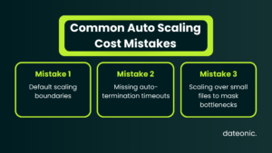Defining Strict Minimum and Maximum Boundaries</b></h3> <p><span style="font-weight: 400;">The foundation of cost control is defining a realistic spread between your compute boundaries. However, architectural constraints vary significantly by compute type.</span></p> <p> </p> <p><span style="font-weight: 400;">For classic Spark clusters, you define a spread of </span><span style="font-weight: 400;">min_workers</span><span style="font-weight: 400;"> and </span><span style="font-weight: 400;">max_workers</span><span style="font-weight: 400;">.</span></p> <p> </p> <ul> <li style="font-weight: 400;" aria-level="1"><b>Minimum boundaries:</b><span style="font-weight: 400;"> Establish the baseline capacity required for your workload to begin execution without waiting for node initialization. Setting this too high incurs idle costs; setting it too low throttles performance.</span></li> <li style="font-weight: 400;" aria-level="1"><b>Maximum boundaries:</b><span style="font-weight: 400;"> This acts as your financial fail-safe. It prevents runaway costs triggered by unoptimized, massive Cartesian join queries.</span></li> </ul> <p> </p> <p><span style="font-weight: 400;">For Databricks Lakebase (PostgreSQL) transactional workloads, capacity is measured in Compute Units (CUs). High Availability (HA) configurations carry specific auto-scaling spread limits. [VERIFY] Currently, instances deployed in an HA configuration share a strict maximum spread limit of 16 CUs between the minimum and maximum boundaries.</span></p> <p> </p> <p><b>Example Cluster Policy Configuration (Classic Spark):</b></p> <p> </p> <blockquote><p><span style="font-weight: 400;">{</span></p> <p><span style="font-weight: 400;"> „autoscale.min_workers”: {</span></p> <p><span style="font-weight: 400;"> „type”: „fixed”,</span></p> <p><span style="font-weight: 400;"> „value”: 2</span></p> <p><span style="font-weight: 400;"> },</span></p> <p><span style="font-weight: 400;"> „autoscale.max_workers”: {</span></p> <p><span style="font-weight: 400;"> „type”: „fixed”,</span></p> <p><span style="font-weight: 400;"> „value”: 12</span></p> <p><span style="font-weight: 400;"> },</span></p> <p><span style="font-weight: 400;"> „autotermination_minutes”: {</span></p> <p><span style="font-weight: 400;"> „type”: „fixed”,</span></p> <p><span style="font-weight: 400;"> „value”: 15</span></p> <p><span style="font-weight: 400;"> }</span></p> <p><span style="font-weight: 400;">}</span></p></blockquote> <p> </p> <h3><b>2. Enforcing Auto-Termination and Scale-to-Zero</b></h3> <p><span style="font-weight: 400;">It is critical to distinguish between classic auto-termination and Serverless „Scale-to-Zero” features, as they govern different compute paradigms.</span></p> <p> </p> <p><span style="font-weight: 400;">Interactive and development clusters are notorious for draining enterprise budgets when left running after hours. Enforcing a strict auto-termination policy – typically an inactivity timeout of 10 to 15 minutes – instantly eliminates the cost of „zombie” classic Spark clusters.</span></p> <p> </p> <p><span style="font-weight: 400;">Conversely, Databricks Serverless compute and Lakebase offer a true </span><b>Scale-to-Zero</b><span style="font-weight: 400;"> feature, allowing idle endpoints to terminate completely without maintaining a driver node. Production architects must be aware of its specific limitations:</span></p> <p> </p> <ul> <li style="font-weight: 400;" aria-level="1"><b>Lakebase High Availability Constraints:</b><span style="font-weight: 400;"> For transactional workloads running on Databricks Lakebase, Scale-to-Zero is intentionally disabled [VERIFY] for High Availability replicas to ensure continuous uptime.</span></li> <li style="font-weight: 400;" aria-level="1"><b>Cold Starts:</b><span style="font-weight: 400;"> Scaling up from zero introduces latency. The first request will experience a „cold start” delay ranging from 10 to 20 seconds. It should not be used for production applications requiring guaranteed, sub-second response times.</span></li> </ul> <p> </p> <h3><b>3. Utilizing Automated Job Compute vs. All-Purpose Compute</b></h3> <p><span style="font-weight: 400;">One of the most immediate ways to reduce Databricks Unit (DBU) consumption is isolating development from execution. <a href="https://dateonic.com/how-to-run-python-and-sql-files-with-all-purpose-compute/">All-Purpose Compute</a> (interactive clusters used for notebook development) is billed at a significantly higher DBU rate than automated Job Compute.</span></p> <p> </p> <p><span style="font-weight: 400;">Once your AI and data models move from the discovery phase into production, migrate the workloads to automated Job clusters. Job clusters spin up specifically for the duration of the pipeline and terminate immediately upon completion, drastically lowering your overall compute spend.</span></p> <p> </p> <h3><b>4. Leveraging Serverless SQL Warehouses</b></h3> <p><span style="font-weight: 400;">For Chief Data Officers managing Business Intelligence (BI) costs, classic clusters are often inefficient for highly concurrent, ad-hoc query workloads. Serverless SQL Warehouses utilize intelligent auto-scaling that scales up instantly to handle concurrent user queries and rapidly scales down when traffic subsides. Utilizing Serverless SQL minimizes the management overhead of defining strict worker boundaries while drastically reducing idle BI compute costs.</span></p> <p> </p> <h3><b>5. Blending Spot Instances with On-Demand Drivers</b></h3> <p><span style="font-weight: 400;">Cloud providers offer spot instances (AWS Spot, Azure Spot VMs, or GCP Preemptible VMs) at deep discounts, but they carry preemption risks. You can leverage these savings safely by using a mixed instance fleet strategy.</span></p> <p> </p> <p><span style="font-weight: 400;">Always configure your driver node using On-Demand instances. The driver maintains the state of the Spark application; if it is preempted, the entire job fails. Conversely, configure your worker nodes using Spot instances. Ensure your cluster policies are configured to fall back to On-Demand instances if Spot capacity is unavailable in your chosen region. Because Spark is inherently fault-tolerant, if a spot worker is lost, the driver simply recalculates the lost partitions on the remaining nodes, preserving pipeline stability while reducing hardware costs.</span></p> <p> </p> <h3><b>6. Pre-Optimizing Data Before Scaling Compute</b></h3> <p><span style="font-weight: 400;">Auto-scaling should never be used to mask poorly written code or unoptimized data pipelines. A common performance bottleneck is „metadata overhead”—the result of querying large volumes of small files, which forces the cluster to work harder and triggers unnecessary scaling events.</span></p> <p> </p> <p><span style="font-weight: 400;">Before increasing your </span><span style="font-weight: 400;">max_workers</span><span style="font-weight: 400;"> limit, ensure the underlying data layout is optimized. Implementing the </span><span style="font-weight: 400;">OPTIMIZE</span><span style="font-weight: 400;"> command compacts small files, while </span><span style="font-weight: 400;">ZORDER</span><span style="font-weight: 400;"> co-locates related information within the same set of files. By reducing the I/O burden on the cluster, you drastically reduce the need for horizontal scaling. Read more about structured performance tuning on our</span> <a href="https://dateonic.com/blog/"><span style="font-weight: 400;">Technical Blog</span></a><span style="font-weight: 400;">.</span></p> <p> </p> <style type="text/css"> .tg {border-collapse:collapse;border-spacing:0;}<br /> .tg td{border-color:black;border-style:solid;border-width:1px;font-family:Arial, sans-serif;font-size:14px;<br /> overflow:hidden;padding:10px 5px;word-break:normal;}<br /> .tg th{border-color:black;border-style:solid;border-width:1px;font-family:Arial, sans-serif;font-size:14px;<br /> font-weight:normal;overflow:hidden;padding:10px 5px;word-break:normal;}<br /> .tg .tg-baqh{text-align:center;vertical-align:top}<br /> </style> <table class="tg"> <thead> <tr> <th class="tg-baqh"><span style="font-weight: bold; font-style: normal; text-decoration: none; color: #000; background-color: transparent;">Best Practice</span></th> <th class="tg-baqh"><span style="font-weight: bold; font-style: normal; text-decoration: none; color: #000; background-color: transparent;">Cost Impact</span></th> <th class="tg-baqh"><span style="font-weight: bold; font-style: normal; text-decoration: none; color: #000; background-color: transparent;">Performance Impact</span></th> <th class="tg-baqh"><span style="font-weight: bold; font-style: normal; text-decoration: none; color: #000; background-color: transparent;">Implementation Difficulty</span></th> </tr> </thead> <tbody> <tr> <td class="tg-baqh"><span style="font-weight: 400; font-style: normal; text-decoration: none; color: #000; background-color: transparent;">Set Min/Max Worker Limits</span></td> <td class="tg-baqh"><span style="font-weight: 400; font-style: normal; text-decoration: none; color: #000; background-color: transparent;">High</span></td> <td class="tg-baqh"><span style="font-weight: 400; font-style: normal; text-decoration: none; color: #000; background-color: transparent;">Positive</span></td> <td class="tg-baqh"><span style="font-weight: 400; font-style: normal; text-decoration: none; color: #000; background-color: transparent;">Low</span></td> </tr> <tr> <td class="tg-baqh"><span style="font-weight: 400; font-style: normal; text-decoration: none; color: #000; background-color: transparent;">Enable Auto-Termination</span></td> <td class="tg-baqh"><span style="font-weight: 400; font-style: normal; text-decoration: none; color: #000; background-color: transparent;">Very High</span></td> <td class="tg-baqh"><span style="font-weight: 400; font-style: normal; text-decoration: none; color: #000; background-color: transparent;">Neutral</span></td> <td class="tg-baqh"><span style="font-weight: 400; font-style: normal; text-decoration: none; color: #000; background-color: transparent;">Very Low</span></td> </tr> <tr> <td class="tg-baqh"><span style="font-weight: 400; font-style: normal; text-decoration: none; color: #000; background-color: transparent;">Use Job Compute</span></td> <td class="tg-baqh"><span style="font-weight: 400; font-style: normal; text-decoration: none; color: #000; background-color: transparent;">High</span></td> <td class="tg-baqh"><span style="font-weight: 400; font-style: normal; text-decoration: none; color: #000; background-color: transparent;">Neutral</span></td> <td class="tg-baqh"><span style="font-weight: 400; font-style: normal; text-decoration: none; color: #000; background-color: transparent;">Low</span></td> </tr> <tr> <td class="tg-baqh"><span style="font-weight: 400; font-style: normal; text-decoration: none; color: #000; background-color: transparent;">Adopt Serverless SQL</span></td> <td class="tg-baqh"><span style="font-weight: 400; font-style: normal; text-decoration: none; color: #000; background-color: transparent;">High</span></td> <td class="tg-baqh"><span style="font-weight: 400; font-style: normal; text-decoration: none; color: #000; background-color: transparent;">Positive</span></td> <td class="tg-baqh"><span style="font-weight: 400; font-style: normal; text-decoration: none; color: #000; background-color: transparent;">Medium</span></td> </tr> <tr> <td class="tg-baqh"><span style="font-weight: 400; font-style: normal; text-decoration: none; color: #000; background-color: transparent;">Use Spot Workers</span></td> <td class="tg-baqh"><span style="font-weight: 400; font-style: normal; text-decoration: none; color: #000; background-color: transparent;">Very High</span></td> <td class="tg-baqh"><span style="font-weight: 400; font-style: normal; text-decoration: none; color: #000; background-color: transparent;">Slight Risk</span></td> <td class="tg-baqh"><span style="font-weight: 400; font-style: normal; text-decoration: none; color: #000; background-color: transparent;">Medium</span></td> </tr> <tr> <td class="tg-baqh"><span style="font-weight: 400; font-style: normal; text-decoration: none; color: #000; background-color: transparent;">Optimize Data Layout (OPTIMIZE/ZORDER)</span></td> <td class="tg-baqh"><span style="font-weight: 400; font-style: normal; text-decoration: none; color: #000; background-color: transparent;">High</span></td> <td class="tg-baqh"><span style="font-weight: 400; font-style: normal; text-decoration: none; color: #000; background-color: transparent;">Very Positive</span></td> <td class="tg-baqh"><span style="font-weight: 400; font-style: normal; text-decoration: none; color: #000; background-color: transparent;">Medium</span></td> </tr> </tbody> </table> <p> </p> <h2><b>Enterprise Governance and Cost Monitoring</b></h2> <p><span style="font-weight: 400;">Scaling optimizations are only effective if they can be measured. For engineering leads, the ultimate source of truth for DBU consumption is the </span><span style="font-weight: 400;">system.billing.usage</span><span style="font-weight: 400;"> table.</span></p> <p> </p> <p><span style="font-weight: 400;">This system table provides the raw, metered record of everything Databricks charges for. To achieve true cost observability, engineering teams must:</span></p> <p> </p> <ul> <li style="font-weight: 400;" aria-level="1"><span style="font-weight: 400;">Enforce strict resource tagging across all workspaces to attribute costs to specific teams and projects.</span></li> <li style="font-weight: 400;" aria-level="1"><span style="font-weight: 400;">Set up automated budget alerts linked to specific cluster policies.</span></li> <li style="font-weight: 400;" aria-level="1"><span style="font-weight: 400;">Query the </span><span style="font-weight: 400;">system.billing.usage</span><span style="font-weight: 400;"> table, joining it with pricing data and workload metadata, to audit the exact financial impact of auto-scaling behaviors.</span></li> </ul> <p> </p> <h2><b>Conclusion: Scaling with a Databricks Consulting Partner</b></h2> <p><span style="font-weight: 400;">Databricks auto-scaling is a powerful capability, but translating elasticity into actual enterprise cost savings requires specialized engineering. Default settings will not protect you from metadata bottlenecks, misconfigured instance fleets, or idle waste.</span></p> <p> </p> <p><span style="font-weight: 400;">As an Official Databricks Consulting Partner, Dateonic specializes in structuring production-grade MLOps, executing complex Data Warehouse migrations, and building scalable Lakehouse architectures. We help enterprises enforce robust data governance through Unity Catalog and optimize cluster compute to deliver reliable performance without the bloat.</span></p> <p> </p> <p><span style="font-weight: 400;">Stop paying for idle capacity and start running production-ready AI.</span> <a href="https://dateonic.com/contact-us/"><span style="font-weight: 400;">Talk to a Databricks expert today</span></a><span style="font-weight: 400;"> to optimize your platform.</span></p> <p> </p> <h2><b>FAQ</b></h2> <p> </p> <p><b>What metrics does Databricks use to trigger auto-scaling?</b></p> <p> </p> <p><span style="font-weight: 400;">Databricks does not solely look at CPU usage. It analyzes Spark scheduler signals, including pending tasks, available task slots, node idleness, and memory consumption.</span></p> <p> </p> <p><b>Can Databricks clusters scale down to zero?</b></p> <p> </p> <p><span style="font-weight: 400;">Yes, but the mechanism depends on the compute type. Classic Spark clusters can use auto-termination to shut down after a period of inactivity. Databricks Serverless and Lakebase compute utilize a true Scale-to-Zero feature, though it introduces a „cold start” latency and is disabled for Lakebase High Availability configurations.</span></p> <p> </p> <p><b>Why is my Databricks bill so high if auto-scaling is enabled?</b></p> <p> </p> <p><span style="font-weight: 400;">High bills are often the result of using expensive All-Purpose Compute for automated tasks, lacking aggressive auto-termination policies, failing to utilize Serverless SQL Warehouses for BI, or suffering from data layout issues (like the small file problem) that force the cluster to scale up unnecessarily.</span></p> <p> </p> <p><b>What is the difference between Job Compute and All-Purpose Compute?</b></p> <p> </p> <p><span style="font-weight: 400;">All-Purpose Compute is designed for interactive, multi-user development and carries a higher DBU price. Job Compute is designed for automated, scheduled workloads and is billed at a lower, more cost-effective rate.</span></p> </div> </div> </div> </div> </div> </div> <div data-elementor-type="footer" data-elementor-id="126" class="elementor elementor-126 elementor-location-footer" data-elementor-post-type="elementor_library"> <div class="elementor-element elementor-element-13e0d1f e-flex e-con-boxed e-con e-parent" data-id="13e0d1f" data-element_type="container"> <div class="e-con-inner"> <div class="elementor-element elementor-element-1c45384 e-con-full e-flex elementor-invisible e-con e-child" data-id="1c45384" data-element_type="container" data-settings="{"background_background":"classic","animation":"fadeInUp"}"> <div class="elementor-element elementor-element-4d5df70 e-con-full e-flex e-con e-child" data-id="4d5df70" data-element_type="container"> <div class="elementor-element elementor-element-4c918d8 elementor-widget__width-inherit elementor-invisible elementor-widget elementor-widget-heading" data-id="4c918d8" data-element_type="widget" data-settings="{"_animation":"fadeInUp"}" data-widget_type="heading.default"> <div class="elementor-widget-container"> <h2 class="elementor-heading-title elementor-size-default">Let's talk about your project!</h2> </div> </div> </div> <div class="elementor-element elementor-element-7de8d50 e-con-full e-flex e-con e-child" data-id="7de8d50" data-element_type="container"> <div class="elementor-element elementor-element-66979f1 elementor-invisible elementor-widget elementor-widget-button" data-id="66979f1" data-element_type="widget" data-settings="{"_animation":"fadeInUp","_animation_delay":700}" data-widget_type="button.default"> <div class="elementor-widget-container"> <div class="elementor-button-wrapper"> <a class="elementor-button elementor-button-link elementor-size-sm" href="https://dateonic.com/contact-us/"> <span class="elementor-button-content-wrapper"> <span class="elementor-button-text">Contact Us</span> </span> </a> </div> </div> </div> </div> </div> </div> </div> <div class="elementor-element elementor-element-541c38a4 e-flex e-con-boxed e-con e-parent" data-id="541c38a4" data-element_type="container" data-settings="{"background_background":"classic"}"> <div class="e-con-inner"> <div class="elementor-element elementor-element-16728b33 e-con-full e-flex e-con e-child" data-id="16728b33" data-element_type="container"> <div class="elementor-element elementor-element-127a768e e-con-full e-flex e-con e-child" data-id="127a768e" data-element_type="container"> <div class="elementor-element elementor-element-7423752b elementor-widget elementor-widget-heading" data-id="7423752b" data-element_type="widget" data-widget_type="heading.default"> <div class="elementor-widget-container"> <h3 class="elementor-heading-title elementor-size-default">Explore</h3> </div> </div> <div class="elementor-element elementor-element-28b68075 elementor-icon-list--layout-traditional elementor-list-item-link-full_width elementor-widget elementor-widget-icon-list" data-id="28b68075" data-element_type="widget" data-widget_type="icon-list.default"> <div class="elementor-widget-container"> <ul class="elementor-icon-list-items"> <li class="elementor-icon-list-item"> <a href="https://dateonic.com/"> <span class="elementor-icon-list-text">Home</span> </a> </li> <li class="elementor-icon-list-item"> <a href="https://dateonic.com/about-us"> <span class="elementor-icon-list-text">About</span> </a> </li> <li class="elementor-icon-list-item"> <a href="https://dateonic.com/case-studies"> <span class="elementor-icon-list-text">Projects</span> </a> </li> <li class="elementor-icon-list-item"> <a href="https://dateonic.com/blog"> <span class="elementor-icon-list-text">Blog</span> </a> </li> <li class="elementor-icon-list-item"> <a href="https://dateonic.com/contact-us/"> <span class="elementor-icon-list-text">Contact us</span> </a> </li> </ul> </div> </div> </div> <div class="elementor-element elementor-element-2d2cf75a e-con-full e-flex e-con e-child" data-id="2d2cf75a" data-element_type="container"> <div class="elementor-element elementor-element-60a21c4a elementor-widget elementor-widget-heading" data-id="60a21c4a" data-element_type="widget" data-widget_type="heading.default"> <div class="elementor-widget-container"> <h3 class="elementor-heading-title elementor-size-default">Portfolio</h3> </div> </div> <div class="elementor-element elementor-element-27aa64ea elementor-icon-list--layout-traditional elementor-list-item-link-full_width elementor-widget elementor-widget-icon-list" data-id="27aa64ea" data-element_type="widget" data-widget_type="icon-list.default"> <div class="elementor-widget-container"> <ul class="elementor-icon-list-items"> <li class="elementor-icon-list-item"> <a href="https://dateonic.com/case-studies/snowflake-to-databricks-migration/"> <span class="elementor-icon-list-text">Snowflakes to Databricks migration</span> </a> </li> <li class="elementor-icon-list-item"> <a href="https://dateonic.com/case-studies-v2/smart-energy-optimization/"> <span class="elementor-icon-list-text">Smart Energy Optimization</span> </a> </li> <li class="elementor-icon-list-item"> <a href="https://dateonic.com/case-studies/skyfare-dynamics/"> <span class="elementor-icon-list-text">Dynamic AI Pricing for Airlines</span> </a> </li> <li class="elementor-icon-list-item"> <a href="https://dateonic.com/case-studies/transglobal-logistics/"> <span class="elementor-icon-list-text">Big Data in Logistics</span> </a> </li> <li class="elementor-icon-list-item"> <a href="https://dateonic.com/case-studies-v2/cloud-powered-analytics/"> <span class="elementor-icon-list-text">Cloud Powered Analytics</span> </a> </li> <li class="elementor-icon-list-item"> <a href="https://dateonic.com/case-studies-v2/fintech-transformation-with-databricks/"> <span class="elementor-icon-list-text">Fintech Transformation with Databricks</span> </a> </li> </ul> </div> </div> </div> <div class="elementor-element elementor-element-71fdbc8 e-con-full e-flex e-con e-child" data-id="71fdbc8" data-element_type="container"> <div class="elementor-element elementor-element-a110d41 elementor-widget elementor-widget-heading" data-id="a110d41" data-element_type="widget" data-widget_type="heading.default"> <div class="elementor-widget-container"> <h3 class="elementor-heading-title elementor-size-default">Industries</h3> </div> </div> <div class="elementor-element elementor-element-8fae269 elementor-icon-list--layout-traditional elementor-list-item-link-full_width elementor-widget elementor-widget-icon-list" data-id="8fae269" data-element_type="widget" data-widget_type="icon-list.default"> <div class="elementor-widget-container"> <ul class="elementor-icon-list-items"> <li class="elementor-icon-list-item"> <a href="https://dateonic.com/accelerating-automotive-innovation-with-big-data-and-ai/"> <span class="elementor-icon-list-text">Automotive</span> </a> </li> <li class="elementor-icon-list-item"> <a href="https://dateonic.com/ai-and-big-data-solutions-for-aviation/"> <span class="elementor-icon-list-text">Aviation</span> </a> </li> <li class="elementor-icon-list-item"> <a href="https://dateonic.com/fintech"> <span class="elementor-icon-list-text">Fintech</span> </a> </li> <li class="elementor-icon-list-item"> <a href="https://dateonic.com/healthcare-transformation-with-big-data-ai-and-databricks/"> <span class="elementor-icon-list-text">Healthcare</span> </a> </li> <li class="elementor-icon-list-item"> <a href="https://dateonic.com/big-data-and-ai-in-logistics-with-databricks/"> <span class="elementor-icon-list-text">Logistics</span> </a> </li> <li class="elementor-icon-list-item"> <a href="https://dateonic.com/smart-manufacturing-with-big-data-ai-and-databricks/"> <span class="elementor-icon-list-text">Manufacturing</span> </a> </li> <li class="elementor-icon-list-item"> <a href="https://dateonic.com/ai-and-big-data-in-ocean-freight-navigating-maritime-logistics-with-databricks/"> <span class="elementor-icon-list-text">Ocean Freight</span> </a> </li> <li class="elementor-icon-list-item"> <a href="https://dateonic.com/revolutionizing-real-estate-with-big-data-ai-and-databricks/"> <span class="elementor-icon-list-text">Real Estate</span> </a> </li> <li class="elementor-icon-list-item"> <a href="https://dateonic.com/retail/"> <span class="elementor-icon-list-text">Retail</span> </a> </li> </ul> </div> </div> </div> <div class="elementor-element elementor-element-6393d80c e-con-full e-flex e-con e-child" data-id="6393d80c" data-element_type="container"> <div class="elementor-element elementor-element-294e1869 elementor-widget elementor-widget-heading" data-id="294e1869" data-element_type="widget" data-widget_type="heading.default"> <div class="elementor-widget-container"> <h3 class="elementor-heading-title elementor-size-default">Follow us</h3> </div> </div> <div class="elementor-element elementor-element-59a25646 elementor-icon-list--layout-traditional elementor-list-item-link-full_width elementor-widget elementor-widget-icon-list" data-id="59a25646" data-element_type="widget" data-widget_type="icon-list.default"> <div class="elementor-widget-container"> <ul class="elementor-icon-list-items"> <li class="elementor-icon-list-item"> <a href="https://www.linkedin.com/company/dateonic"> <span class="elementor-icon-list-text">LinkedIn</span> </a> </li> <li class="elementor-icon-list-item"> <a href="https://github.com/dateonic"> <span class="elementor-icon-list-text">GitHub</span> </a> </li> <li class="elementor-icon-list-item"> <a href="https://www.youtube.com/@dateonic"> <span class="elementor-icon-list-text">Youtube</span> </a> </li> </ul> </div> </div> </div> </div> </div> </div> <div class="elementor-element elementor-element-40dae2fd e-flex e-con-boxed e-con e-parent" data-id="40dae2fd" data-element_type="container" data-settings="{"background_background":"classic"}"> <div class="e-con-inner"> <div class="elementor-element elementor-element-16fd32e e-con-full e-flex e-con e-child" data-id="16fd32e" data-element_type="container"> <div class="elementor-element elementor-element-1be7d43b elementor-widget elementor-widget-text-editor" data-id="1be7d43b" data-element_type="widget" data-widget_type="text-editor.default"> <div class="elementor-widget-container"> <p>DATEONIC SP. Z O.O. registered at Ludna 2, 00-406 Warsaw, Poland</p> </div> </div> <div class="elementor-element elementor-element-5c70b88 elementor-widget elementor-widget-text-editor" data-id="5c70b88" data-element_type="widget" data-widget_type="text-editor.default"> <div class="elementor-widget-container"> <p>Copyright © 2025 dateonic.com</p> </div> </div> </div> <div class="elementor-element elementor-element-68d9c17a e-con-full e-flex e-con e-child" data-id="68d9c17a" data-element_type="container"> <div class="elementor-element elementor-element-2023120c elementor-widget__width-auto elementor-widget elementor-widget-button" data-id="2023120c" data-element_type="widget" data-widget_type="button.default"> <div class="elementor-widget-container"> <div class="elementor-button-wrapper"> <a class="elementor-button elementor-button-link elementor-size-sm" href="https://dateonic.com/privacy-policy/"> <span class="elementor-button-content-wrapper"> <span class="elementor-button-text">Privacy Policy</span> </span> </a> </div> </div> </div> <div class="elementor-element elementor-element-2ece220a elementor-widget__width-auto elementor-widget elementor-widget-button" data-id="2ece220a" data-element_type="widget" data-widget_type="button.default"> <div class="elementor-widget-container"> <div class="elementor-button-wrapper"> <a class="elementor-button elementor-button-link elementor-size-sm" href="https://dateonic.com/privacy-policy/"> <span class="elementor-button-content-wrapper"> <span class="elementor-button-text">Terms & Services</span> </span> </a> </div> </div> </div> </div> </div> </div> </div> <script type="speculationrules"> {"prefetch":[{"source":"document","where":{"and":[{"href_matches":"/"},{"not":{"href_matches":["/wp-.php","/wp-admin/","/wp-content/uploads/","/wp-content/","/wp-content/plugins/","/wp-content/themes/hello-elementor/","/\\?(.+)"]}},{"not":{"selector_matches":"a[rel~=\"nofollow\"]"}},{"not":{"selector_matches":".no-prefetch, .no-prefetch a"}}]},"eagerness":"conservative"}]} </script> <script> const lazyloadRunObserver = () => { const lazyloadBackgrounds = document.querySelectorAll( `.e-con.e-parent:not(.e-lazyloaded)` ); const lazyloadBackgroundObserver = new IntersectionObserver( ( entries ) => { entries.forEach( ( entry ) => { if ( entry.isIntersecting ) { let lazyloadBackground = entry.target; if( lazyloadBackground ) { lazyloadBackground.classList.add( 'e-lazyloaded' ); } lazyloadBackgroundObserver.unobserve( entry.target ); } }); }, { rootMargin: '200px 0px 200px 0px' } ); lazyloadBackgrounds.forEach( ( lazyloadBackground ) => { lazyloadBackgroundObserver.observe( lazyloadBackground ); } ); }; const events = [ 'DOMContentLoaded', 'elementor/lazyload/observe', ]; events.forEach( ( event ) => { document.addEventListener( event, lazyloadRunObserver ); } ); </script> <script id="hello-theme-frontend-js" src="https://dateonic.com/wp-content/themes/hello-elementor/assets/js/hello-frontend.js?ver=3.4.4"></script> <script id="elementor-webpack-runtime-js" src="https://dateonic.com/wp-content/plugins/elementor/assets/js/webpack.runtime.min.js?ver=3.30.4"></script> <script id="elementor-frontend-modules-js" src="https://dateonic.com/wp-content/plugins/elementor/assets/js/frontend-modules.min.js?ver=3.30.4"></script> <script id="jquery-ui-core-js" src="https://dateonic.com/wp-includes/js/jquery/ui/core.min.js?ver=1.13.3"></script> <script id="elementor-frontend-js-before"> var elementorFrontendConfig = {"environmentMode":{"edit":false,"wpPreview":false,"isScriptDebug":false},"i18n":{"shareOnFacebook":"Udost\u0119pnij na Facebooku","shareOnTwitter":"Udost\u0119pnij na Twitterze","pinIt":"Przypnij","download":"Pobierz","downloadImage":"Pobierz obraz","fullscreen":"Tryb pe\u0142noekranowy","zoom":"Powi\u0119ksz","share":"Udost\u0119pnij","playVideo":"Odtw\u00f3rz wideo","previous":"Poprzednie","next":"Nast\u0119pne","close":"Zamknij","a11yCarouselPrevSlideMessage":"Poprzedni slajd","a11yCarouselNextSlideMessage":"Nast\u0119pny slajd","a11yCarouselFirstSlideMessage":"To jest pierwszy slajd","a11yCarouselLastSlideMessage":"To jest ostatni slajd","a11yCarouselPaginationBulletMessage":"Id\u017a do slajdu"},"is_rtl":false,"breakpoints":{"xs":0,"sm":480,"md":768,"lg":1025,"xl":1440,"xxl":1600},"responsive":{"breakpoints":{"mobile":{"label":"Mobilny Pionowy","value":767,"default_value":767,"direction":"max","is_enabled":true},"mobile_extra":{"label":"Mobilny Poziomy","value":880,"default_value":880,"direction":"max","is_enabled":false},"tablet":{"label":"Portret tabletu","value":1024,"default_value":1024,"direction":"max","is_enabled":true},"tablet_extra":{"label":"Ekran tabletu","value":1200,"default_value":1200,"direction":"max","is_enabled":false},"laptop":{"label":"Laptop","value":1366,"default_value":1366,"direction":"max","is_enabled":false},"widescreen":{"label":"Szeroki ekran","value":2400,"default_value":2400,"direction":"min","is_enabled":false}},"hasCustomBreakpoints":false},"version":"3.30.4","is_static":false,"experimentalFeatures":{"e_font_icon_svg":true,"additional_custom_breakpoints":true,"container":true,"theme_builder_v2":true,"hello-theme-header-footer":true,"nested-elements":true,"e_element_cache":true,"home_screen":true,"global_classes_should_enforce_capabilities":true,"cloud-library":true,"e_opt_in_v4_page":true},"urls":{"assets":"https:\/\/dateonic.com\/wp-content\/plugins\/elementor\/assets\/","ajaxurl":"https:\/\/dateonic.com\/wp-admin\/admin-ajax.php","uploadUrl":"https:\/\/dateonic.com\/wp-content\/uploads"},"nonces":{"floatingButtonsClickTracking":"b2d9cd65c6"},"swiperClass":"swiper","settings":{"page":[],"editorPreferences":[]},"kit":{"body_background_background":"classic","active_breakpoints":["viewport_mobile","viewport_tablet"],"global_image_lightbox":"yes","lightbox_enable_counter":"yes","lightbox_enable_fullscreen":"yes","lightbox_enable_zoom":"yes","lightbox_enable_share":"yes","lightbox_title_src":"title","lightbox_description_src":"description","hello_header_logo_type":"title","hello_header_menu_layout":"horizontal","hello_footer_logo_type":"logo"},"post":{"id":2797,"title":"Databricks%20Auto%20Scaling%20Best%20Practices%20for%20Cost%20Control%20-%20dateonic.","excerpt":"","featuredImage":"https:\/\/dateonic.com\/wp-content\/uploads\/2026\/06\/databricksautoscalingbestpracticesforcostcontrolbanner-1024x480.png"}}; //# sourceURL=elementor-frontend-js-before </script> <script id="elementor-frontend-js" src="https://dateonic.com/wp-content/plugins/elementor/assets/js/frontend.min.js?ver=3.30.4"></script> <script id="smartmenus-js" src="https://dateonic.com/wp-content/plugins/elementor-pro/assets/lib/smartmenus/jquery.smartmenus.min.js?ver=1.2.1"></script> <script id="e-sticky-js" src="https://dateonic.com/wp-content/plugins/elementor-pro/assets/lib/sticky/jquery.sticky.min.js?ver=3.30.1"></script> <script id="elementor-pro-webpack-runtime-js" src="https://dateonic.com/wp-content/plugins/elementor-pro/assets/js/webpack-pro.runtime.min.js?ver=3.30.1"></script> <script id="wp-hooks-js" src="https://dateonic.com/wp-includes/js/dist/hooks.min.js?ver=7496969728ca0f95732d"></script> <script id="wp-i18n-js" src="https://dateonic.com/wp-includes/js/dist/i18n.min.js?ver=781d11515ad3d91786ec"></script> <script id="wp-i18n-js-after"> wp.i18n.setLocaleData( { 'text direction\u0004ltr': [ 'ltr' ] } ); //# sourceURL=wp-i18n-js-after </script> <script id="elementor-pro-frontend-js-before"> var ElementorProFrontendConfig = {"ajaxurl":"https:\/\/dateonic.com\/wp-admin\/admin-ajax.php","nonce":"ad5efdb01c","urls":{"assets":"https:\/\/dateonic.com\/wp-content\/plugins\/elementor-pro\/assets\/","rest":"https:\/\/dateonic.com\/wp-json\/"},"settings":{"lazy_load_background_images":true},"popup":{"hasPopUps":false},"shareButtonsNetworks":{"facebook":{"title":"Facebook","has_counter":true},"twitter":{"title":"Twitter"},"linkedin":{"title":"LinkedIn","has_counter":true},"pinterest":{"title":"Pinterest","has_counter":true},"reddit":{"title":"Reddit","has_counter":true},"vk":{"title":"VK","has_counter":true},"odnoklassniki":{"title":"OK","has_counter":true},"tumblr":{"title":"Tumblr"},"digg":{"title":"Digg"},"skype":{"title":"Skype"},"stumbleupon":{"title":"StumbleUpon","has_counter":true},"mix":{"title":"Mix"},"telegram":{"title":"Telegram"},"pocket":{"title":"Pocket","has_counter":true},"xing":{"title":"XING","has_counter":true},"whatsapp":{"title":"WhatsApp"},"email":{"title":"Email"},"print":{"title":"Print"},"x-twitter":{"title":"X"},"threads":{"title":"Threads"}},"facebook_sdk":{"lang":"pl_PL","app_id":""},"lottie":{"defaultAnimationUrl":"https:\/\/dateonic.com\/wp-content\/plugins\/elementor-pro\/modules\/lottie\/assets\/animations\/default.json"}}; //# sourceURL=elementor-pro-frontend-js-before </script> <script id="elementor-pro-frontend-js" src="https://dateonic.com/wp-content/plugins/elementor-pro/assets/js/frontend.min.js?ver=3.30.1"></script> <script id="pro-elements-handlers-js" src="https://dateonic.com/wp-content/plugins/elementor-pro/assets/js/elements-handlers.min.js?ver=3.30.1"></script> <script id="wp-emoji-settings" type="application/json"> {"baseUrl":"https://s.w.org/images/core/emoji/17.0.2/72x72/","ext":".png","svgUrl":"https://s.w.org/images/core/emoji/17.0.2/svg/","svgExt":".svg","source":{"concatemoji":"https://dateonic.com/wp-includes/js/wp-emoji-release.min.js?ver=7.0.1"}} </script> <script type="module"> /! This file is auto-generated / const a=JSON.parse(document.getElementById("wp-emoji-settings").textContent),o=(window._wpemojiSettings=a,"wpEmojiSettingsSupports"),s=["flag","emoji"];function i(e){try{var t={supportTests:e,timestamp:(new Date).valueOf()};sessionStorage.setItem(o,JSON.stringify(t))}catch(e){}}function c(e,t,n){e.clearRect(0,0,e.canvas.width,e.canvas.height),e.fillText(t,0,0);t=new Uint32Array(e.getImageData(0,0,e.canvas.width,e.canvas.height).data);e.clearRect(0,0,e.canvas.width,e.canvas.height),e.fillText(n,0,0);const a=new Uint32Array(e.getImageData(0,0,e.canvas.width,e.canvas.height).data);return t.every((e,t)=>e===a[t])}function p(e,t){e.clearRect(0,0,e.canvas.width,e.canvas.height),e.fillText(t,0,0);var n=e.getImageData(16,16,1,1);for(let e=0;e<n.data.length;e++)if(0!==n.data[e])return!1;return!0}function u(e,t,n,a){switch(t){case"flag":return n(e,"\ud83c\udff3\ufe0f\u200d\u26a7\ufe0f","\ud83c\udff3\ufe0f\u200b\u26a7\ufe0f")?!1:!n(e,"\ud83c\udde8\ud83c\uddf6","\ud83c\udde8\u200b\ud83c\uddf6")&&!n(e,"\ud83c\udff4\udb40\udc67\udb40\udc62\udb40\udc65\udb40\udc6e\udb40\udc67\udb40\udc7f","\ud83c\udff4\u200b\udb40\udc67\u200b\udb40\udc62\u200b\udb40\udc65\u200b\udb40\udc6e\u200b\udb40\udc67\u200b\udb40\udc7f");case"emoji":return!a(e,"\ud83e\u1fac8")}return!1}function f(e,t,n,a){let r;const o=(r="undefined"!=typeof WorkerGlobalScope&&self instanceof WorkerGlobalScope?new OffscreenCanvas(300,150):document.createElement("canvas")).getContext("2d",{willReadFrequently:!0}),s=(o.textBaseline="top",o.font="600 32px Arial",{});return e.forEach(e=>{s[e]=t(o,e,n,a)}),s}function r(e){var t=document.createElement("script");t.src=e,t.defer=!0,document.head.appendChild(t)}a.supports={everything:!0,everythingExceptFlag:!0},new Promise(t=>{let n=function(){try{var e=JSON.parse(sessionStorage.getItem(o));if("object"==typeof e&&"number"==typeof e.timestamp&&(new Date).valueOf()<e.timestamp+604800&&"object"==typeof e.supportTests)return e.supportTests}catch(e){}return null}();if(!n){if("undefined"!=typeof Worker&&"undefined"!=typeof OffscreenCanvas&&"undefined"!=typeof URL&&URL.createObjectURL&&"undefined"!=typeof Blob)try{var e="postMessage("+f.toString()+"("+[JSON.stringify(s),u.toString(),c.toString(),p.toString()].join(",")+"));",a=new Blob([e],{type:"text/javascript"});const r=new Worker(URL.createObjectURL(a),{name:"wpTestEmojiSupports"});return void(r.onmessage=e=>{i(n=e.data),r.terminate(),t(n)})}catch(e){}i(n=f(s,u,c,p))}t(n)}).then(e=>{for(const n in e)a.supports[n]=e[n],a.supports.everything=a.supports.everything&&a.supports[n],"flag"!==n&&(a.supports.everythingExceptFlag=a.supports.everythingExceptFlag&&a.supports[n]);var t;a.supports.everythingExceptFlag=a.supports.everythingExceptFlag&&!a.supports.flag,a.supports.everything||((t=a.source||{}).concatemoji?r(t.concatemoji):t.wpemoji&&t.twemoji&&(r(t.twemoji),r(t.wpemoji)))}); //# sourceURL=https://dateonic.com/wp-includes/js/wp-emoji-loader.min.js </script> </body> </html>