
Performance work in Databricks often starts with the wrong question. Teams resize a cluster, force a broadcast join, or add caching before checking where the job is actually spending time. Sometimes that helps. Sometimes it simply makes an inefficient query more expensive.
A slow workload might be waiting for compute, scanning files it could have skipped, spilling during a shuffle, or running code that falls back from Photon to Spark. Those problems need different fixes. Treat the five techniques below as an order of operations rather than a ranking.
1. Measure the workload before tuning it
Choose a real query, job, or pipeline that matters to users. For SQL warehouses and serverless compute, Query Profile is the best place to start. It shows the executed operators, time spent, memory use, rows processed, and I/O.
Full table scans, exploding joins, large shuffles, and one unusually slow operator are usually easy to spot there. For classic jobs and all-purpose compute, use the Spark UI and compute metrics.
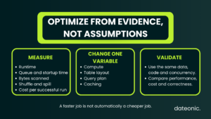
For a useful baseline, record:
- total runtime, including queue and startup time;
- rows and bytes read, plus the amount of data pruned;
- shuffle read and write, disk spill, and uneven task durations;
- output row counts and data correctness;
- compute consumption and the cost of a successful run.
Query history is also available through system.query.history for supported compute. You can compare it with usage from system.billing.usage, provided the relevant job, warehouse, and tag metadata is present.
One fast run proves little. Keep the data, code, concurrency, and compute configuration stable, then repeat the test after each meaningful change. If caching or startup time may affect the result, compare cold and repeated runs separately.
2. Benchmark the right compute option and check Photon
Databricks recommends serverless compute for most new workloads. It removes cluster provisioning and lets the platform handle startup and scaling. Still, serverless is not an automatic answer.
Some workloads need networking, libraries, data sources, or runtime features that are not supported, so check the current serverless requirements and limitations before moving production jobs.
Photon accelerates supported SQL, DataFrame, ETL, and stateless streaming operations. It is already enabled on serverless compute and SQL warehouses.
For classic compute created through an API, set Photon explicitly so that an automated deployment does not depend on a UI default.
The important detail is coverage. Unsupported operations fall back to the Spark runtime, while UDF-heavy or RDD-based code can limit how much of a job Photon executes.
Query Profile and the Spark UI show that split. If the expected improvement is missing, inspect the plan before changing the cluster again.
Compare the same workload on the compute options that are genuinely available to you. Runtime matters, but so do queue time, failures, resource use, and cost per successful run. A larger cluster that finishes earlier is not necessarily the better configuration.
3. Let Databricks manage table layout where it can
Many apparent compute problems begin with table layout. When a query opens too many small files or cannot skip irrelevant data, adding workers only attacks the symptom.
Current Delta Lake best practices favor Unity Catalog managed tables with predictive optimization and liquid clustering. Predictive optimization runs ANALYZE, OPTIMIZE, and VACUUM when eligible tables are likely to benefit.
Liquid clustering is the recommended layout for new tables and replaces traditional partitioning and ZORDER.
For an eligible managed table, automatic clustering can be enabled with:
ALTER TABLE main.analytics.orders CLUSTER BY AUTO;
ALTER TABLE main.analytics.orders ENABLE PREDICTIVE OPTIMIZATION;
CLUSTER BY AUTO is not a drop-in setting for every table. Confirm the runtime, table eligibility, and protocol compatibility first, especially if another engine or external Delta client reads the same data.
Predictive optimization also uses billable serverless jobs compute. Before enabling automated VACUUM, check whether the current retention policy provides enough history for time travel and recovery.
Once predictive optimization is active, remove duplicate scheduled OPTIMIZE jobs. External tables and older workloads may still need optimized writes, auto compaction, or manual OPTIMIZE, but base that decision on table history and scan behavior.
A single target file size is not appropriate for every table.
4. Give the optimizer current statistics
Rules such as “broadcast every table below this size” age badly. Join performance also depends on filters, data distribution, executor memory, concurrency, and the rest of the physical plan.
The cost-based optimizer needs current table and column statistics to choose between those plans. Predictive optimization collects them for eligible managed tables.
Elsewhere, collect the statistics manually and inspect the plan:
ANALYZE TABLE main.analytics.orders COMPUTE STATISTICS FOR ALL COLUMNS;

EXPLAIN
SELECT c.segment, SUM(o.net_amount)
FROM main.analytics.orders AS o
JOIN main.analytics.customers AS c
  ON o.customer_id = c.customer_id
WHERE o.order_date >= current_date() - INTERVAL 1 MONTH
GROUP BY c.segment;
EXPLAIN shows whether estimates are available. Query Profile or the Spark UI then shows what actually ran. Large differences between estimated and actual rows often explain a poor join choice. A
lso check whether filters are applied before the join and whether one key produces most of the shuffle.
Adaptive Query Execution is enabled by default. It can change join strategies, combine small shuffle partitions, and mitigate skew using information collected during execution.
Where supported, use auto-optimized shuffle instead of carrying an old partition count from another workload:
SET spark.sql.shuffle.partitions = auto;
Only add an explicit broadcast hint or a manual skew workaround when the executed plan shows that the automatic strategy is still wrong. The same dimension table may be safe to broadcast today and too large after data growth or a change in concurrency.
5. Treat caching as the finishing move
Caching is last on this list for a reason. It helps when the same data is read repeatedly, but it will not repair a full table scan, missing statistics, or poor clustering.
The old Delta Cache name has been replaced by Databricks disk cache. On classic compute, workers with local SSD storage can cache Parquet and Delta files automatically. Databricks invalidates stale entries when the underlying files change.
Some older caching advice no longer applies. Databricks documents that CACHE SELECT is ignored on SQL warehouses and on Databricks Runtime 14.2 and later, where the platform uses an enhanced disk-caching algorithm.
Spark caching is separate. It can still make sense when the same DataFrame is reused within one job, but creating and retaining that cache consumes memory and compute.
Autoscaling matters too. If a worker holding Spark-cached partitions is removed, those partitions must be read or calculated again. Test caching with the scaling policy used in production, not on an artificially stable cluster.
Compare cold and warm runs, then ask whether the production access pattern looks the same. If a dataset is normally read only once, a faster second run improves the benchmark rather than the workload.
What a defensible result looks like
After an optimization, you should be able to name the workload, data snapshot, compute configuration, and metrics used in the comparison.
Record runtime and cost, but also verify the output and failure behavior. That evidence is more useful than a generic claim that Photon, liquid clustering, or caching makes Databricks “faster.”
No single setting solves every performance problem. Start with the executed plan, fix the layer that is doing unnecessary work, and rerun the same test.
If you need help tracing a bottleneck across compute, queries, and table layout, explore Dateonic’s Databricks consulting services or talk to a Databricks architect.