Querying Files and Writing to Delta Tables in Databricks

Author:

Date:

24 maja, 2025

Ever found yourself juggling different file formats—CSV, JSON, Parquet—trying to make sense of them and write clean, performant tables?

Maybe your SQL queries get messy, your schema breaks mid-pipeline, or your tables just aren’t fast enough for analytics. Efficiently reading files, transforming data, and writing it to optimized Delta tables is one of the most essential (and often frustrating) skills in modern data engineering.

In this guide, I’ll walk you through practical, real-world techniques for handling files and tables in Databricks—from reading raw files to writing high-performance Delta tables with partitioning, schema evolution, and more.

Supported File Formats in Databricks

Databricks offers robust support for various file formats, each with its own advantages and trade-offs. Understanding these differences helps you make informed decisions about which format to use for your specific use case.

Popular File Formats Comparison

Format	Advantages	Disadvantages	Best Use Cases
Parquet	– Columnar storage – High compression – Schema evolution – Predicate pushdown support – Excellent query performance	– Not human-readable – More complex than CSV/JSON	– Analytics workloads – Large datasets – Complex queries
CSV	– Human-readable – Universal compatibility – Simple structure – Easy to create	– No schema enforcement – Poor compression – Slower queries – No nested data support	– Simple data exchange – Legacy systems integration – Small datasets
JSON	– Human-readable – Schema flexibility – Nested structure support – Wide compatibility	– Verbose format – Less efficient storage – Slower than Parquet – Variable parsing performance	– Semi-structured data – API responses – Document storage

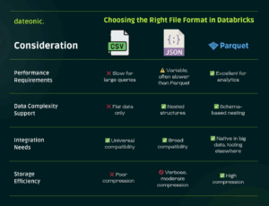
Key Considerations When Choosing a Format

Selecting the right file format in Databricks depends on factors like query performance, data structure, compatibility, and storage efficiency. To help you quickly compare these trade-offs across CSV, JSON, and Parquet, I’ve summarized the differences in the following infographic:

How to Read Files in Databricks

Databricks provides several methods to read files, with options to customize the reading process according to your data’s specific characteristics.

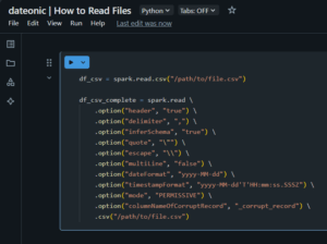
CSV Files

# Basic CSV reading

df_csv = spark.read.csv(„/path/to/file.csv”)

# CSV with options

df_csv_with_options = spark.read.option(„header”, „true”) \

                              .option(„delimiter”, „,”) \

                              .option(„inferSchema”, „true”) \

                              .csv(„/path/to/file.csv”)

# Comprehensive CSV example with all common options

df_csv_complete = spark.read \

    .option(„header”, „true”) \

    .option(„delimiter”, „,”) \

    .option(„inferSchema”, „true”) \

    .option(„quote”, „\””) \

    .option(„escape”, „\\”) \

    .option(„multiLine”, „false”) \

    .option(„dateFormat”, „yyyy-MM-dd”) \

    .option(„timestampFormat”, „yyyy-MM-dd’T’HH:mm:ss.SSSZ”) \

    .option(„mode”, „PERMISSIVE”) \

    .option(„columnNameOfCorruptRecord”, „_corrupt_record”) \

    .csv(„/path/to/file.csv”)

Key CSV reading options:

header: Specifies if the first line is a header (true/false)
delimiter: Character separating fields (comma, tab, pipe, etc.)
inferSchema: Automatically detect column types (true/false)
multiLine: Support records spanning multiple lines (true/false)
mode: How to handle corrupt records (PERMISSIVE, DROPMALFORMED, FAILFAST)

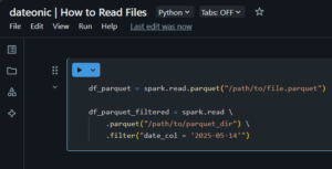
Parquet Files

# Basic Parquet reading

df_parquet = spark.read.parquet(„/path/to/file.parquet”)

# Parquet with partition pruning (improves performance)

df_parquet_filtered = spark.read \

.parquet(„/path/to/parquet_dir”) \

.filter(„date_col = '2025-05-14′”)

JSON Files

# Basic JSON reading

df_json = spark.read.json(„/path/to/file.json”)

# JSON with options for multi-line JSON records

df_json_multiline = spark.read \

    .option(„multiLine”, „true”) \

    .option(„mode”, „PERMISSIVE”) \

    .json(„/path/to/file.json”)

Reading Multiple Files with Wildcards

# Read all CSV files in a directory

df_multiple = spark.read \

    .option(„header”, „true”) \

    .option(„inferSchema”, „true”) \

    .csv(„/path/to/csv_files/*.csv”)

Querying File Data Using SQL

After reading files, you can leverage Spark SQL to analyze your data effectively. This approach combines the flexibility of SQL with Databricks’ distributed computing power.

Creating Temporary Views

Temporary views allow you to query your dataframes using SQL syntax:

# Create a temporary view from our dataframe

df_csv_with_options.createOrReplaceTempView(„customer_data”)

# Now query using SQL

result_df = spark.sql(„””

    SELECT

        customer_id,

        SUM(purchase_amount) as total_spent,

        COUNT(*) as transaction_count

    FROM

        customer_data

    WHERE

        purchase_date >= '2025-01-01′

    GROUP BY

        customer_id

    ORDER BY

        total_spent DESC

„””)

# Display the results

display(result_df)

Creating Global Temporary Views

Global temporary views persist across multiple Spark sessions within the same cluster:

# Create a global temporary view

df_parquet.createOrReplaceGlobalTempView(„product_catalog”)

# Query the global temporary view (note the global_temp database prefix)

result_global = spark.sql(„””

SELECT * FROM global_temp.product_catalog

WHERE product_category = 'Electronics’

„””)

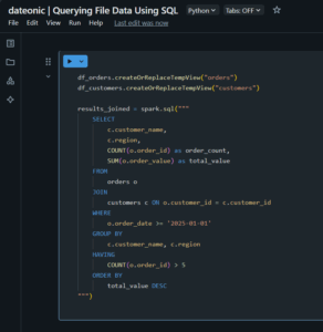
SQL Subqueries and Joins with Temporary Views

# Create multiple views

df_orders.createOrReplaceTempView(„orders”)

df_customers.createOrReplaceTempView(„customers”)

# Complex SQL with joins

results_joined = spark.sql(„””

    SELECT

        c.customer_name,

        c.region,

        COUNT(o.order_id) as order_count,

        SUM(o.order_value) as total_value

    FROM

        orders o

    JOIN

        customers c ON o.customer_id = c.customer_id

    WHERE

        o.order_date >= '2025-01-01′

    GROUP BY

        c.customer_name, c.region

    HAVING

        COUNT(o.order_id) > 5

    ORDER BY

        total_value DESC

„””)

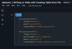
Writing to Table with Creating Table from File

Once you’ve processed your data, you’ll often want to persist it as a Delta table for optimized storage and future queries.

Creating a Delta Table from a DataFrame

# Basic table creation

df_processed.write \

    .format(„delta”) \

    .mode(„overwrite”) \

    .saveAsTable(„customer_analytics”)

# Table creation with partitioning

df_processed.write \

    .format(„delta”) \

    .partitionBy(„year”, „month”) \

    .mode(„overwrite”) \

    .saveAsTable(„customer_analytics_partitioned”)

Using INSERT OVERWRITE with SQL

# First, create or replace a temporary view

df_processed.createOrReplaceTempView(„processed_data”)

# Then use SQL to insert into a table

spark.sql(„””

    INSERT OVERWRITE TABLE customer_analytics

    SELECT

        customer_id,

        product_id,

        purchase_date,

        amount,

        YEAR(purchase_date) as year,

        MONTH(purchase_date) as month

    FROM

        processed_data

    WHERE

        amount > 0

„””)

Handling Schema Evolution

When your data schema changes over time, Delta tables can adapt seamlessly:

# Enable schema evolution

spark.sql(„SET spark.databricks.delta.schema.autoMerge.enabled = true”)

# Write with schema evolution enabled

df_new_schema.write \

    .format(„delta”) \

    .option(„mergeSchema”, „true”) \

    .mode(„append”) \

    .saveAsTable(„customer_analytics”)

Creating Tables with Advanced Options

# Create a Delta table with additional options

spark.sql(„””

    CREATE TABLE IF NOT EXISTS sales_performance

    USING DELTA

    PARTITIONED BY (region, date)

    LOCATION '/mnt/data/sales_performance’

    COMMENT 'Sales performance data for analytics’

    AS

    SELECT * FROM processed_sales_data

„””)

Optimizing Delta Tables After Writing

To ensure optimal query performance, run optimization commands after substantial writes:

# Optimize (compaction)

spark.sql(„OPTIMIZE customer_analytics”)

# Z-ORDER optimization for faster filtering

spark.sql(„OPTIMIZE customer_analytics ZORDER BY (customer_id, purchase_date)”)

What’s Next?

Now that you’ve mastered querying files and writing to Delta tables in Databricks, you might want to explore these related topics:

Understanding Medallion Architecture in Databricks and How to Implement It – Learn how to structure your data processing workflows in layers for better quality and management
What is Unity Catalog and How It Keeps Your Data Secure – Discover how to enhance data governance and security in your Databricks environment
What is Lakehouse Architecture and How It Differs from Data Lake and Data Warehouse – Gain a deeper understanding of the architecture that powers Databricks
What are Workflows in Databricks and How Do They Work – Learn how to orchestrate your data processing pipelines effectively
Getting Started with Databricks: Creating Your First Cluster – If you’re new to Databricks, start with the basics of setting up your environment

Take Your Data Engineering Skills to the Next Level

Ready to transform your data engineering capabilities with Databricks? Our team of certified data experts can help you implement best practices, optimize your workflows, and maximize the value of your data assets.