Databricks MLflow Tutorial Step-by-Step

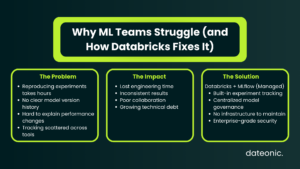
ML teams waste hours every week trying to reproduce experiments, track which model version made it to production, or explain why a run two weeks ago yielded better results than today’s. Without proper tracking infrastructure, those hours compound into serious engineering debt.

 

Databricks solves this with a fully managed, hosted version of MLflow – built directly into the platform with enterprise-grade security, high availability, and native workspace integration. Unlike self-hosted MLflow, you get experiment and run management out of the box, governed by Unity Catalog, with no additional infrastructure to maintain.

 

MLflow on Databricks is built around four core capabilities:

 

• Tracking – log parameters, metrics, and artifacts from every run
• Model Registry – centralized hub for versioning and governance
• Model Serving – deploy models to REST API endpoints via Mosaic AI
• Monitoring – capture and analyze live inference data

 

This Databricks MLflow tutorial covers the full workflow on AWS – from environment setup through model deployment. It’s the practical AWS counterpart to Azure-focused Databricks guides; if you’re curious how the two clouds compare, see our breakdown of Databricks on Azure and AWS – Key Differences.

 

Target audience: data engineers and ML practitioners running Databricks on AWS who want a repeatable, production-grade experiment tracking workflow.

 

 

Before You Start This Databricks MLflow Tutorial

 

Before writing a single line of code, confirm you have the following:

 

• Databricks workspace on AWS – the free Community Edition covers most steps in this guide; note that Mosaic AI Model Serving endpoints cannot be created on Community Edition, so model deployment requires a full workspace
• Cluster on Databricks Runtime 17.3 LTS ML or above – this runtime ships with scikit-learn, MLflow, and Optuna pre-installed, so no manual library installs are needed
• Unity Catalog privileges – you’ll need USE_CATALOG, USE_SCHEMA, CREATE_TABLE, and CREATE_MODEL on the target catalog and schema
• Python familiarity – intermediate-level; no advanced ML background required for this walkthrough
• Optional: a local IDE connected via a Databricks Personal Access Token, if you prefer developing outside the notebook interface

 

Cluster configuration has a direct impact on cost and performance. For guidance on keeping things efficient, see Optimizing Clusters in Databricks: Performance, Cost, and Best Practices.

 

Key MLflow Concepts You Need to Know

 

Before diving into the tutorial steps, it helps to have these four concepts clear in your head:

 

Run – a single execution of your model training code. Each run automatically captures the environment, plus anything you explicitly log: parameters, metrics, tags, and output files.

 

Experiment – a named collection of related runs. Think of it as the container for all the iterations you do on one modeling problem.

 

Logged Model – a distinct entity that persists across runs and environments. It stores links to artifacts, metrics, parameters, and the code that produced it. This is what eventually gets registered and deployed.

 

Model Registry – the centralized governance hub, integrated with Unity Catalog in modern Databricks workspaces. It provides lineage, cross-workspace access, and access controls.

 

Version note: Databricks currently runs MLflow 3 as its default version. The examples in this tutorial are written against MLflow 3 APIs.

 

For a deeper look at how Unity Catalog underpins model governance, see Databricks Unity Catalog vs Hive Metastore – understanding the difference matters when you set registry URIs and permissions.

 

Area	Without MLflow	With Databricks MLflow
Experiment tracking	Manual, inconsistent	Automatic, structured
Reproducibility	Hard to replicate runs	Fully reproducible
Model versioning	Ad hoc naming	Centralized registry
Collaboration	Fragmented	Shared workspace
Debugging	Time-consuming	Traceable history
Governance	Limited	Unity Catalog integration

 

Databricks MLflow Tutorial: Step-by-Step Walkthrough

 

Step 1 – Set Up Your MLflow Experiment

Open a new notebook in your Databricks AWS workspace. One important convenience: when working inside a Databricks notebook, MLflow is already authenticated to your workspace – no additional credential setup is required.

 

Start by pointing MLflow at Unity Catalog as your model registry, then define the catalog and schema where models will be stored:

 

import mlflow

 

# Use Unity Catalog as the model registry

mlflow.set_registry_uri(„databricks-uc”)

 

# Set the catalog and schema for model registration

CATALOG = „your_catalog”

SCHEMA = „your_schema”

 

# Create or set the experiment

mlflow.set_experiment(f”/Users/your_email@example.com/wine_quality_experiment”)

 

Using databricks-uc as the registry URI is what connects your runs to Unity Catalog governance rather than the legacy Hive Metastore.

 

Step 2 – Load and Prepare Data

This tutorial uses the UCI Wine Quality dataset – 11 physicochemical features with a quality score from 1 to 10. It’s a well-known, reproducible reference that maps cleanly to a regression task.

 

Load the data and save a copy to a Unity Catalog table so it’s governed alongside your models:

 

import pandas as pd

from sklearn.model_selection import train_test_split

 

# Load dataset

df = pd.read_csv(

    „https://archive.ics.uci.edu/ml/machine-learning-databases/wine-quality/winequality-red.csv”,

    sep=„;”

)

 

# Save to Unity Catalog for lineage tracking

spark_df = spark.createDataFrame(df)

spark_df.write.mode(„overwrite”).saveAsTable(f”{CATALOG}.{SCHEMA}.wine_quality_raw”)

 

# Split for training

X = df.drop(„quality”, axis=1)

y = df[„quality”]

X_train, X_test, y_train, y_test = train_test_split(X, y, test_size=0.2, random_state=42)

 

Saving the raw data to a Unity Catalog table is a small step that pays off significantly: it creates a lineage link between your training data and any models you later register. For a complete guide to getting data into Databricks on AWS, see How to Ingest Data into Databricks from AWS S3.

 

Step 3 – Track an Experiment Run

MLflow tracking lets you log parameters, metrics, tags, and artifacts from each training run. The with mlflow.start_run(): context manager ensures the run is properly opened and closed, even if an exception occurs.

 

from sklearn.ensemble import RandomForestRegressor

from sklearn.metrics import mean_squared_error, r2_score

import numpy as np

 

# Enable autologging for scikit-learn (logs params, metrics, and model automatically)

mlflow.sklearn.autolog()

 

with mlflow.start_run(run_name=„random_forest_baseline”):

    # Define and train model

    params = {„n_estimators”: 100, „max_depth”: 6, „random_state”: 42}

    model = RandomForestRegressor(**params)

    model.fit(X_train, y_train)

 

    # Evaluate

    predictions = model.predict(X_test)

    rmse = np.sqrt(mean_squared_error(y_test, predictions))

    r2 = r2_score(y_test, predictions)

 

    # Log manually if not relying solely on autolog

    mlflow.log_params(params)

    mlflow.log_metrics({„rmse”: rmse, „r2”: r2})

    mlflow.sklearn.log_model(model, artifact_path=„model”)

 

mlflow.sklearn.autolog() is the fastest path for scikit-learn pipelines – it captures hyperparameters, evaluation metrics, and the serialized model without manual logging calls. You can still add manual log_metrics calls on top for custom evaluation logic.

 

Key things being logged per run:

 

• Parameters – model hyperparameters (n_estimators, max_depth, etc.)
• Metrics – RMSE, R², or any custom evaluation score
• Artifacts – the serialized model, feature importance plots, or any output file
• Tags – optional metadata like team name, data version, or ticket ID

 

Step 4 – Compare Runs in the MLflow UI

Once you have two or more runs, navigate to Experiments in the left sidebar under the AI/ML section. The experiment page lets you compare runs side by side and drill into individual run details.

 

The most useful comparison view is the parallel coordinates chart – it draws a line per run across axes for each hyperparameter and metric, making it immediately clear which combinations drive better results. To use it:

 

1. Select two or more runs using the checkboxes
2. Click Compare in the top toolbar
3. Switch to the Parallel Coordinates tab

 

This view becomes especially valuable once you introduce hyperparameter sweeps (Optuna or Hyperopt), where you might have 50–100 runs to analyze.

 

Step 5 – Register the Model in Unity Catalog

Once you’ve identified the best run, register it in Unity Catalog. You need USE_CATALOG privilege on the catalog and USE_SCHEMA, CREATE_TABLE, and CREATE_MODEL privileges on the schema before this will succeed.

 

# Get the run ID of your best run

best_run_id = „paste_run_id_here”

 

model_uri = f”runs:/{best_run_id}/model”

model_name = f”{CATALOG}.{SCHEMA}.wine_quality_rf”

 

# Register in Unity Catalog

registered_model = mlflow.register_model(

    model_uri=model_uri,

    name=model_name

)

 

print(f”Model registered: {registered_model.name}, version: {registered_model.version}”)

 

After registration, the model appears in the Unity Catalog explorer under your chosen catalog and schema. From there you can add aliases (e.g., @champion, @challenger), view lineage back to the training data and notebook, and manage access policies. For help structuring a Unity Catalog implementation across your organization, see Databricks Unity Catalog Implementation Services & Consulting.

 

Step 6 – Deploy via Mosaic AI Model Serving

With the model registered in Unity Catalog, deployment to a REST endpoint is a one-click operation from the Model Registry UI – or a single API call if you prefer automation:

 

import requests

 

# Deploy via REST API (requires a full workspace, not Community Edition)

headers = {

    „Authorization”: f”Bearer {databricks_token}”,

    „Content-Type”: „application/json”

}

 

endpoint_config = {

    „name”: „wine-quality-endpoint”,

    „config”: {

        „served_models”: [{

            „model_name”: f”{CATALOG}.{SCHEMA}.wine_quality_rf”,

            „model_version”: „1”,

            „workload_size”: „Small”,

            „scale_to_zero_enabled”: True

        }]

    }

}

 

response = requests.post(

    f”{databricks_host}/api/2.0/serving-endpoints”,

    headers=headers,

    json=endpoint_config

)

 

Mosaic AI Model Serving automatically captures requests and responses at the endpoint, which feeds directly into model monitoring. A few things worth knowing about serving:

 

• Not available on Community Edition – you need a full Databricks workspace on AWS
• Scale to zero – endpoints can be configured to scale down when idle, reducing cost
• Automatic request logging – inference logs are written back to a Delta table for monitoring

 

MLflow 3 on AWS: What’s New

 

Databricks ships MLflow 3 as its current default, and a few features are worth highlighting for teams building production MLOps workflows.

 

Deployment Jobs manage the full model lifecycle – evaluation, approval gates, and deployment steps – as governed workflows backed by Unity Catalog. Every event in the lifecycle is written to an activity log, giving you a complete audit trail from experiment to production.

 

MLflow Tracing extends observability beyond classic ML into LLM and agent use cases. It records inputs, outputs, and metadata at each step of an inference chain, making it possible to debug multi-step GenAI pipelines with the same tooling you use for traditional models.

 

For teams that are already running MLflow tracking for classic ML and starting to explore LLM-based features, MLflow 3’s tracing capabilities mean you don’t need a separate observability stack – the same experiment-tracking UI covers both.

 

Take Your MLflow Workflow Further with Dateonic

 

You now have a working end-to-end Databricks MLflow tutorial covering the full lifecycle on AWS: experiment setup, data ingestion, run tracking, model registration in Unity Catalog, and deployment via Mosaic AI Model Serving.

 

Getting to this point in a notebook is straightforward. Getting it into production – with proper governance, automated retraining pipelines, model monitoring, and cost controls – is where architecture decisions matter significantly.

 

Dateonic is an official Databricks implementation partner, helping enterprise teams build complete, AI-ready data platforms across the full Lakehouse stack. If your team is standardizing its MLOps practice on Databricks, explore how we approach it: Databricks MLflow Implementation Partner: Standardizing MLOps.

 

For broader architecture and implementation support, contact us or explore the full Dateonic technical blog for related Lakehouse, MLOps, and data engineering guides.